.jpg)
数据挖掘:作业 03
数据挖掘:实验三 Logistic 回归
代码地址:Github
实验目的和要求
通过在Python中的实例应用,分析掌握Logistic回归分析方法的基本原理,加深对Logistic回归分析算法的理解,并掌握将算法应用于实际的方法、步骤。
实验内容和原理
- 在Python中完成Logistic回归算法模型的数据输入、参数设置;
- 对Python中Logistic回归算法的实例数据输出结果进行分析。
操作方法和实验步骤
Question1
用Python语言实现Logistic回归算法,下载数据集telco.csv,数据集包括“region”(地区)、“tenure”(服务的月数)、“age”(年龄)以及“churn”(客户流失)等42个字段。属性churn的取值为“0”或者“1”,其中“0”表示没有流失,“1”表示流失。,要求完成:
-
利用梯度下降法计算Logistic回归模型的参数。
-
利用牛顿法计算Logistic回归模型的参数。(hint: Logistic回归分析方法求解中的负对数极大似然函数的二阶Hessian矩阵如下:
$$
H = X^TDX,D=diag(d_1,d_2,...,d_m),d_i=g(x^T_iw)(1-g(x^T_iw)),\
diag(d_1,d_2,...,d_m)代表以d_1,d_2,...,d_m为对角元的对角矩阵
$$ -
在Logistic回归模型中加入正则化项,实现计算过程。
Question2
对数据的某一列乘上一个很大的数(比如100000),再分别调用梯度上升法与牛顿法计算Logistic回归模型的参数,你有什么发现?
实验结果和分析
逻辑回归梯度下降法
主要代码:
# The sigmoid function
def Sigmoid(z):
return float(1.0 / float((1.0 + np.exp(-1.0 * z))))
def Hypothesis(theta, x):
z = 0
for i in range(len(theta)):
z += x[i] * theta[i]
return Sigmoid(z)
def Cost_Function(X, Y, theta, m):
sumOfErrors = 0
for i in range(m):
xi = X[i]
hi = Hypothesis(theta, xi)
if Y[i] == 1:
error = Y[i] * np.log(hi)
elif Y[i] == 0:
error = (1 - Y[i]) * np.log(1 - hi)
sumOfErrors += error
const = -1 / m
J = const * sumOfErrors
print('cost is ', J)
return J
def Cost_Function_Derivative(X, Y, theta, j, m, alpha):
sumErrors = 0
for i in range(m):
xi = X[i]
xij = xi[j]
hi = Hypothesis(theta, X[i])
error = (hi - Y[i]) * xij
sumErrors += error
m = len(Y)
constant = float(alpha) / float(m)
return constant * sumErrors
def Gradient_Descent(X, Y, theta, m, alpha):
new_theta = []
for j in range(len(theta)):
CFDerivative = Cost_Function_Derivative(X, Y, theta, j, m, alpha)
new_theta_value = theta[j] - CFDerivative
new_theta.append(*new_theta_value)
return new_theta
def Declare_Winner(theta):
score = 0
length = len(X_test)
for i in range(length):
prediction = round(Hypothesis(X_test[i], theta))
answer = y_test[i]
if prediction == answer:
score += 1
my_score = float(score) / float(length)
print('Your score: ', my_score)
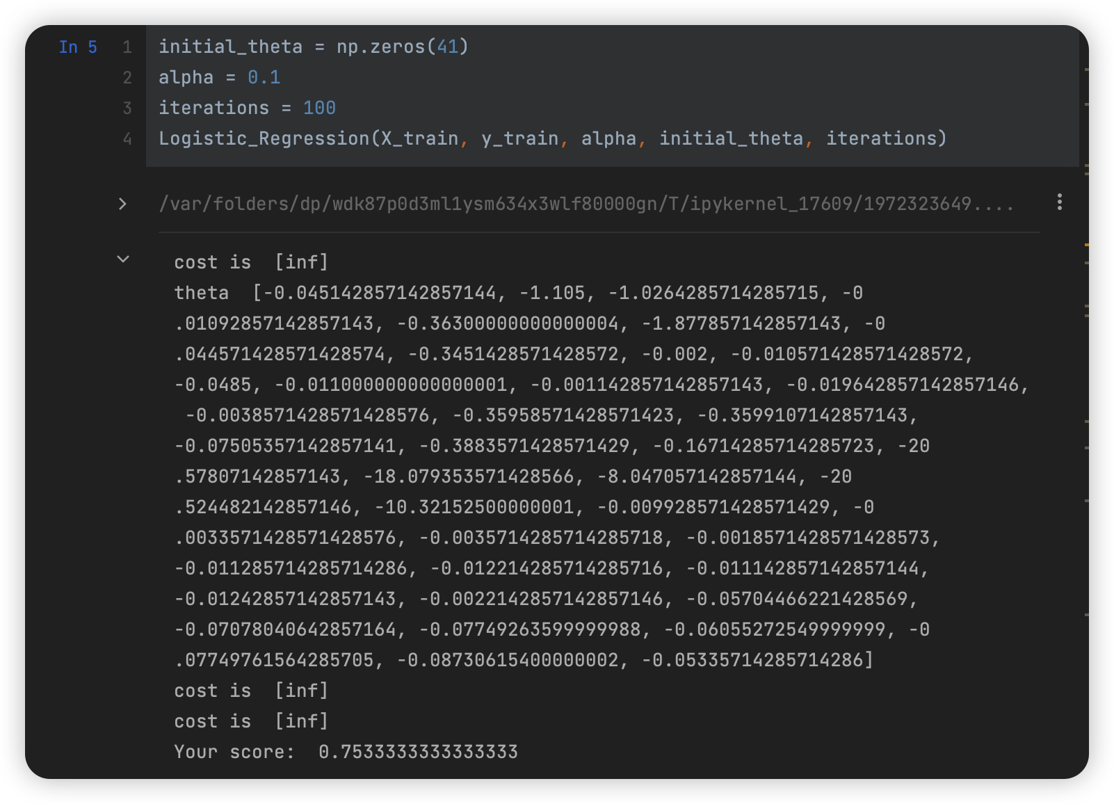
def Logistic_Regression(X, Y, alpha, theta, num_iters):
m = len(Y)
for x in range(num_iters):
new_theta = Gradient_Descent(X, Y, theta, m, alpha)
theta = new_theta
if x % 100 == 0:
Cost_Function(X, Y, theta, m)
print('theta ', theta)
print('cost is ', Cost_Function(X, Y, theta, m))
Declare_Winner(theta)
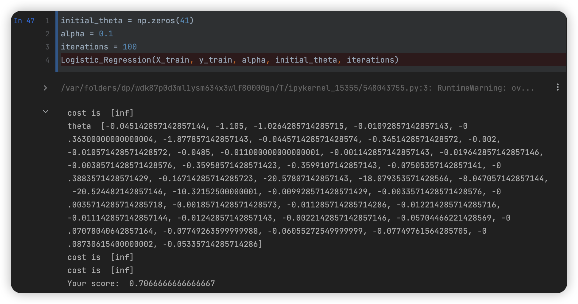
- 这里也因为数据内的异常值从而出现了【inf】
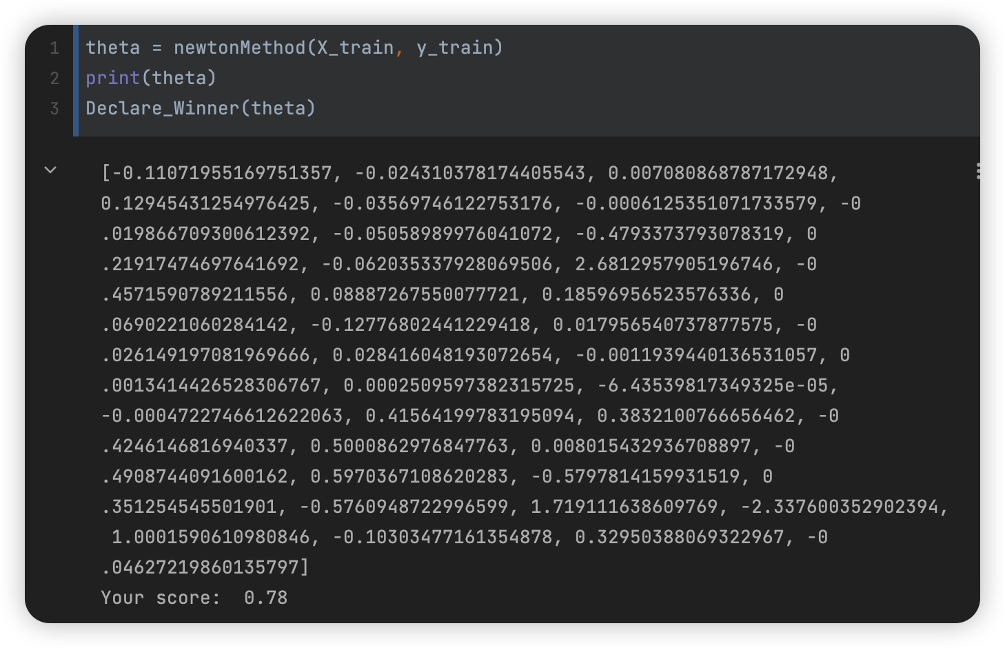
逻辑回归牛顿法
# sigmod函数
def sigmoid(x):
    return 1.0 / (1+math.exp(-x))


# 计算hessian矩阵
def computeHessianMatrix(data, hypothesis):
    hessianMatrix = []
    n = len(data)

    for i in range(n):
        row = []
        for j in range(n):
            row.append(-data[i]*data[j]*(1-hypothesis)*hypothesis)
        hessianMatrix.append(row)
    return hessianMatrix


# 计算两个向量的点积
def computeDotProduct(a, b):
    if len(a) != len(b):
        return False
    n = len(a)
    dotProduct = 0
    for i in range(n):
        dotProduct += a[i] * b[i]
    return dotProduct


# 计算两个向量的和
def computeVectPlus(a, b):
    if len(a) != len(b):
        return False
    n = len(a)
    sum = []
    for i in range(n):
        sum.append(a[i]+b[i])
    return sum


# 计算某个向量的n倍
def computeTimesVect(vect, n):
    nTimesVect = []
    for i in range(len(vect)):
        nTimesVect.append(*(n * vect[i]))
    return nTimesVect


# 牛顿法
def newtonMethod(dataMat, labelMat, iterNum=10):
    m = len(dataMat)  # 训练集个数
    n = len(dataMat[0])  # 数据特征纬度
    theta = [0.0] * n

    while (iterNum):
        gradientSum = [0.0] * n
        hessianMatSum = [[0.0] * n] * n
        for i in range(m):
            try:
                hypothesis = sigmoid(computeDotProduct(dataMat[i], theta))
            except:
                continue
            error = labelMat[i] - hypothesis
            gradient = computeTimesVect(dataMat[i], error / m)
            gradientSum = computeVectPlus(gradientSum, gradient)
            hessian = computeHessianMatrix(dataMat[i], hypothesis / m)
            for j in range(n):
                hessianMatSum[j] = computeVectPlus(hessianMatSum[j], hessian[j])

        # 计算hessian矩阵的逆矩阵有可能异常,如果捕获异常则忽略此轮迭代
        try:
            hessianMatInv = np.mat(hessianMatSum).I.tolist()
        except:
            continue
        for k in range(n):
            theta[k] -= computeDotProduct(hessianMatInv[k], gradientSum)

        iterNum -= 1
    return theta
逻辑回归梯度下降法(含正则化项)
def Cost_Function_Derivative(X, Y, theta, j, m, alpha, _lamda):
    sumErrors = 0
    for i in range(m):
        xi = X[i]
        xij = xi[j]
        hi = Hypothesis(theta, X[i])
        error = (hi - Y[i]) * xij
        sumErrors += error
    m = len(Y)
    constant = float(alpha) / float(m) + (_lamda / float(m) * theta[j])
    return constant * sumErrors
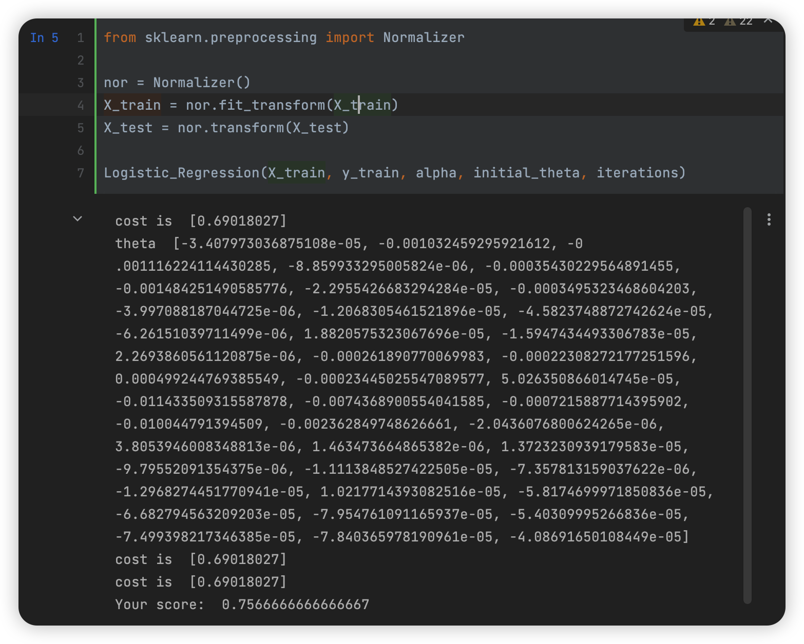
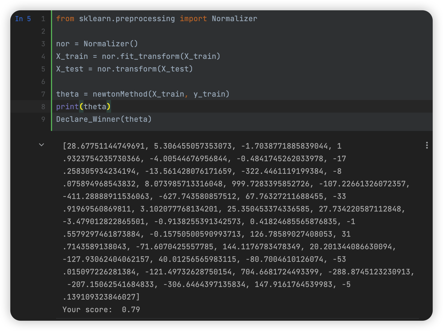
改变数据后使用数据归一化
改变数据后,出现如下问题:
- 时间花费更久
- 拟合速度更快,且不会出现【inf】异常结果
本文是原创文章,采用 CC BY-NC-ND 4.0 协议,完整转载请注明来自 Owen

评论
匿名评论
隐私政策
你无需删除空行,直接评论以获取最佳展示效果